Quantifying Risk in Turbulent Times
- Apr 3, 2020
- 8 min read
Updated: May 11, 2020
Intro
These are turbulent times. After 2008, again we are on the brink of a heavy economic crisis. Needless to say that management boards together with their risk management, financial management and restructuring teams are challenged to move their ships through rough waters. Newspapers are full with terms like black swan, fat-tail risk, 27-sigma events or... what have you? Whatever the situation, extreme events have to be incorporated in any risk management system, or to put it in a more straight way: Risk management systems have to be tried in a way where extreme events are not handled as such extreme anymore.
To begin with, there are rather easy-to-understand and easy-to-implement concepts which can be used to install first vanguards in watching out for high risk events. One of these concepts derives from the basic description of stochastic models, called Kurtosis. Here, I'll have a look at this basic approach and will show kurtosis in the context of real estate share prices, touch the shortcomings of the widespread normal distribution in stochastic risk modeling and discuss why variance can be such a weak risk reflection.
At the end of the article, you find a link showing real estate shares traded at the Frankfurt as well as the Vienna Stock Exchange and covering some of the topics discussed.
Kurtosis
Basically, real data can be described (respectively approximated) by means of a statistical distribution. The distribution itself has four moments:
first moment/ Mean: the average value for all the data points which defines the location of the data distribution
second moment/ Variance: the average distance between the mean and those single data points which defines the scale of the distribution;
third moment/ Skewness: a measure of the asymmetry of the distribution
fourth moment/ Kurtosis: This is the measure of peakiness of a data distribution and signals fat tails. Based on the calculation below, a normal distribution has a kurtosis of zero. Hence, a positive kurtosis reflects a peaked distribution and a negative one equals a flattened distribution
                sum(xi - x_hat)^4
kurtosis = ----------------------------- - 3
              [sum(xi - x_hat)^2]^2


                             sum   ... sum over i=1 to n
                             xi    ... data point
                             x_hat ... average
I'd like to reflect three important applications of kurtosis:
Monitoring data shifts: Kurtosis can be used to monitor shifts in the data distribution. This means that a clear change in the amount of the kurtosis signals a possible change in the data pattern, e.g. the surfacing of fat tails. It is worth noticing that this can be handled with data sets of just moderate size. On the other hand, huge data volume is treated without problems which opens the door to e.g. a vast variety of IoT-applications.
Independent Component Analysis (ICA): ICA is a subsection of the Principal Component Analysis (PCA; for more details: see this article). Basic idea is that in large data sets, there are independent sub-collections of data which are unlikely to have the same means, medians and modes as all the other components of that data set. Therefore, a broad (or fat) tail distribution of the data identified by high kurtosis is an indicator of the presence of multiple components in a complex signal. Moving through the data that yields the highest kurtosis will start to identify those separate sources (subsequent source separation ist then done by Support Vector Machines; but this is a different topic).
Change-point detection in dynamic streaming data: In a massive stream of data, as it is with financial data, it can be beneficial to track a few key parameters which characterize the behavior of the data. Goal is to have an effective early-warning system in place. Kurtosis is a particular effective characterization of the data stream due to its ability to identify the emergence of new behaviors (i.e. new independent components). Even more, this takes place while other key parameter still may produce relatively invariant mean values.
Exchange Traded Real Estate Shares
The further analysis focuses on real estate shares traded at the Frankfurt and at the Vienna Stock Exchange. The portfolio consists of 15 real estate companies. The details of the portfolio can be found here. The graph below shows the daily price changes of all the real estate companies in that portfolio from January 2005 to April 2020.

The distribution of price changes (in other words the frequency of price changes within certain ranges over the monitored time period) gives the typical picture of financial data, i.e.
a more centralized behavior around the mean of the distribution
but equipped with fatter tails.
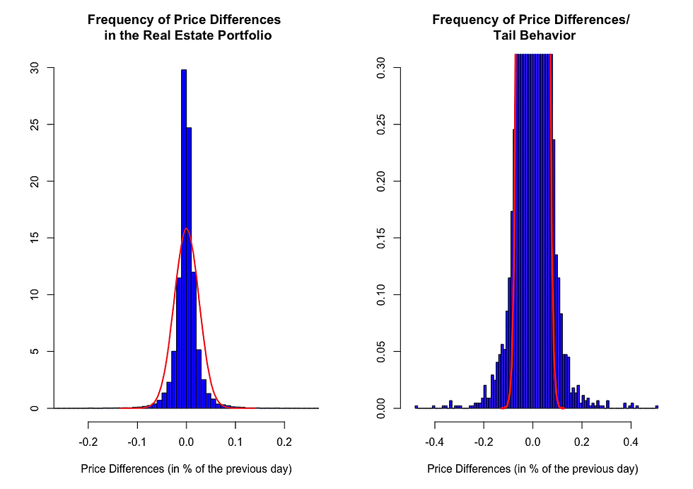
As it is clearly shown, the empirical data (blue bars in the left chart above) can hardly be stochastically approximated by the commonly used normal distribution (red line in the left chart above). The more distinct centering around the mean indicates that, in general, small price movements are the order of the day (compared to what you would expect under normal distribution assumptions). Nevertheless, the heavier tails of the empirical data (blue bars in the right chart above) indicate that price change "surprises" may be expected with a lower probability. Although, those stronger price changes are by far not so rare as it would be simulated by the normal distribution (red line in the right chart above).
This result becomes obvious, considering that the normal distribution is derived only by the first and second moment of the distribution, i.e. the mean and the standard deviation (standard deviation = square root of variance). Skewness and especially kurtosis are not reflected in this framework. To make it more obvious, let's check how the kurtosis and the standard deviation are changing in the course of different market situations. The table below exhibits four different market scenarios based on the data history of the real estate portfolio:
market scenario I: overall market development as from January 2005 including the financial crisis in 2007 to 2009 as well as the current unfolding stock market crisis
market scenario II: a "normal" market scenario without the big shocks of 2007-2009 and 2020
market scenario III: market development from January 2005 till mid of February 2020; so including the financial crisis in 2007 to 2009 but without the current crisis
market scenario IV: market development as from July 2010 (so without the financial crisis in 2007 to 2009 but including the current crisis)
Following results:
                              kurtosis       standard
                                             deviation              --------------------------I--------------I--------------------
market scenario I              35.05            2.52 %
market scenario II             10.07            1.75 %
market scenario III            37.35            2.47 %
market scenario IV             13.97            1.86 %
It is astounding that the standard deviation (resp. variance) as general risk indicator does hardly move in those different circumstances, even when taking heavy market disruptions into account. At the same time, kurtosis shows impressively the peakiness of the distribution and the presence of broader tails, especially when compared to a more 'normal' market environment.
Change of Risk Approach
The overall picture as previously discussed is resembled on a single share level (in this evaluation I've chosen one of the companies in the portfolio). The graph on the left shows the distribution of price changes under 'normal' market conditions (market scenario II in the table above) while the graph on the right includes external shocks (market scenario I from the table above). Empirical data is illustrated with blue bars and the approximation with the normal distribution is presented in a red line.

In both cases, the normal distribution is not an appropriate assumption of the real world. Broader tails are present in both real market scenarios. Though, in the more constrained environment, the empirical data builds out even more significant fat tails while, at the same time, is thinning out around the center. In conclusion, any risk approach with a normal distribution would underestimate the downside risk of a share price development.
The discussion so far indicates that there has to be a more sophisticated way in statistical modeling in order to better approximate the data and to provide a more suitable risk evaluation. One way to do this is via Generalized Lambda Distributions. How exactly this works, would go beyond this article but I would recommend the paper by Steve Su (see references below) for more details. In short, a generalized lambda distribution (GLD) is modeled by taking into account all of the four moments of a distribution (i.e. mean, variance, skewness AND kurtosis). In this example the maximum likelihood method (with three different parameterizations) was used.
The graph below illustrates the much better fit for the Generalized Lambda Distributionthan this would be the case for the normal distribution. The allocation of the market data is described (as always) by the blue bars, the normal distribution is shown in a red line and the GLD is illustrated with a green line.

Looking at the tails of the market data brings the better fit to light (graph is the same as above but the frequency scale is from 0 to just 2). The GLD covers the existence of the heavy tails much better.

But what does this mean in risk terms? Based on the approximation provided by the normal distribution, therisk of facing a negative daily price changeof more than 10% is 0.0001%. You could label this as really rare event. Based on the approximation provided by the generalized lambda distribution, the same event has a probability of 0.64%. According to this, therisk of negative price movements bigger than 10%is6,400-fold higher (!)than before.This is what you call a low probability scenario but definitely not a rare event. Here are some comparisons between those two risk approximations:
                               generalized            normal
daily price movement       lambda distribution      distribution
------------------------I-----------------------I----------------
    more than -20 %               0.20 %            0.00000... %
    more than -10 %               0.64 %            0.0001 %
    more than - 5 %               2.18 %            0.76 %
    more than - 2 %               8.65 %           16.33 %
    negative anyway              49.49 %           49.08 %
Conclusion
There are easy-to-understand and easy-to-implement ways to incorporate early-warnings observation posts in a risk management system. The concept of kurtosis is definitely one way to do that. The capability of handling huge data streams and the potential to identify the emergence of new behavior in a data set are invaluable assets. Kurtosis opens here the gate in the financial data area as well is in the IoT-sector.
Another important subject to note is that an appropriate stochastic modeling in risk management systems is a crucial task. Setting the wrong framework leads on the one hand to ineffective predictive analytics but on the other hand it can have deadly consequences for an enterprise when crisis finally hits.
Not to be misunderstood. Just because an event is rare (in fact: has a low probability) does not mean that from a risk point of view it has to be taken care of. Only when such an event would have a decisive impact on the own system, is it necessary to take a position and neutralize, at least contain the consequences of the cause.
As mentioned in the intro, please find enclosed the following link. This is an easy application showing the share price, the trading volume, daily price changes and the distribution of daily price changes in normal as well as in constrained market conditions for all of the real estate companies in the portfolio.
References
Kurtosis: Four Momentous Uses for the Fourth Moment of Statistical Distributions by Kirk Borne published in Statistic Views/ April 4, 2014
Quantitative Finance Applications in R – 4: Using the Generalized Lambda Distribution to Simulate Market Returns published in Rbloggers/ February 25, 2014
Fitting Single and Mixture of Generalized Lambda Distributions to Data via Discretized and Maximum Likelihood Methods: GLDEX in R by Steve Su published in Journal of Statistical Software, Volume 21 - Issue 9/ October 2007
Kurtosis published in R Tutorial/ n.a.
Flexible distribution modeling with the generalized lambda distribution by Yohan Chalabi and David J Scott and Diethelm Wuertz published in MPRA Munich Personal RePEc Archive/ November 2012
A simple and efficient method for finding the closest generalized lambda distribution to a specific model by Dilanka S. Dedduwakumara, Luke A. Prendergast and Robert G. Staudte published in cogent - mathematics & statistics/ April 4, 2019
Flexible Distribution Modeling with the Generalized Lambda Distribution by Yohan Chalabi and Diethelm Wuertz at ETH Swiss Federal Institute of Technologie Zurich
Families of distributions arising from the quantile of generalized lambda distribution by Mahmoud Aldeni published in Journal of Statistical Distributions and Applications/ November 22, 2017
GLDfunctions: The Generalised Lambda Distribution Family published in rdrr.io/ February 6, 2020
Der Schwarze Schwan by Nassim Nicholas Taleb/ 2007


Comments